Generates flexible plots for longitudinal data, showing either observed values, change from baseline, or both. Supports grouping and faceting.
Usage
lplot(
  df,
  form,
  facet_form = NULL,
  cluster_var = "subject_id",
  baseline_value = NULL,
  xlab = "visit",
  ylab = "measure",
  ylab2 = "measure change",
  title = "Observed Values",
  title2 = "Change from Baseline",
  subtitle = "",
  subtitle2 = "",
  caption = "",
  caption2 = "",
  plot_type = "obs",
  error_type = "bar",
  jitter_width = 0.15,
  color_palette = NULL,
  clinical_mode = FALSE,
  treatment_colors = NULL,
  confidence_interval = NULL,
  summary_statistic = "mean",
  show_sample_sizes = FALSE,
  sample_size_opts = list(),
  theme = "bw",
  publication_ready = FALSE,
  statistical_annotations = FALSE,
  test_method = "parametric",
  p_adjust_method = "BH",
  cov_struct = "auto",
  reference_lines = NULL,
  ribbon_alpha = 0.2,
  ribbon_fill = NULL,
  contrast_display = NULL
)
Arguments
- df
A data frame containing the data to be plotted.
- form
A formula specifying the variables for the x-axis, grouping, and y-axis. Format:
y ~ x | group.- facet_form
A formula specifying the variables for faceting. Format:
facet_y ~ facet_x. Default isNULL.- cluster_var
A character string specifying the name of the cluster variable for grouping within subjects (typically a participant or subject ID).
- baseline_value
The baseline value of the x variable, used to calculate changes. For categorical x variables, this is treated as a level. For continuous x variables, this is treated as a numeric value. If NULL (the default), the function attempts to auto-detect a baseline code from common labels (e.g., 'bl', 'baseline', 'screening') or, for numeric visit variables, uses the minimum value.
- xlab
Label for the x-axis.
- ylab
Label for the y-axis of the observed values plot.
- ylab2
Label for the y-axis of the change values plot.
- title
Title for the observed values plot.
- title2
Title for the change values plot.
- subtitle
Subtitle for the observed values plot.
- subtitle2
Subtitle for the change values plot.
- caption
Caption for the observed values plot.
- caption2
Caption for the change values plot.
- plot_type
Type of plot to return. Options are
"obs"(observed values),"change"(change values), or"both"for combined plots.- error_type
Type of error representation. Options are
"bar"for error bars (vertical lines showing standard error) or"band"for error ribbons (shaded areas around the line).- jitter_width
Numeric. Width of horizontal jitter for error bars when multiple groups are present. Default is 0.1. Set to 0 to disable jittering. Only applies when error_type = "bar".
- color_palette
Optional vector of colors to use for groups. If NULL, default ggplot colors are used.
- clinical_mode
Logical. If TRUE, enables clinical trial defaults (95% CI, sample sizes, clinical colors). Default is FALSE.
- treatment_colors
Character. Predefined color scheme for treatments. Options: "standard" (placebo=grey, active=colors), or NULL.
- confidence_interval
Numeric. Confidence level for error bounds (e.g., 0.95 for 95% CI). If NULL, uses standard error.
- summary_statistic
Character. Type of summary statistic to calculate. Options: "mean" (mean ± CI/SE), "mean_se" (mean ± SE), "median" (median + IQR), or "boxplot" (boxplot summary with quartiles). Default is "mean".
- show_sample_sizes
Logical. If TRUE, shows sample sizes at each timepoint.
- sample_size_opts
List. Options for sample size label appearance. Key option: position = "point" (default, labels next to points) or "table" (color-coded table below x-axis). See
generate_plot()for all available options.- theme
Character. Predefined publication theme with matching colors. Options: "bw", "nejm", "nature", "lancet", "jama", "science", "jco", "fda", or NULL. Defaults to "bw". Applies both typography/layout AND journal-specific color palette automatically.
- publication_ready
Logical. If TRUE, applies publication-ready defaults (professional theme, proper typography, clean styling).
- statistical_annotations
Logical. If TRUE, adds p-values and significance indicators to the plots.
- test_method
Character. Testing approach for group comparisons: "parametric" (t-test / ANOVA, the default), "nonparametric" (Wilcoxon rank-sum / Kruskal-Wallis), or "mmrm" (mixed model for repeated measures with emmeans contrasts; requires the mmrm and emmeans packages).
- p_adjust_method
Character. Multiple comparison correction passed to
stats::p.adjust(). Default is "BH" (Benjamini-Hochberg). Use "none" to disable adjustment.- cov_struct
Character. Covariance structure for MMRM (only used when test_method = "mmrm"). Options: "auto" (unstructured for <= 10 timepoints, compound symmetry otherwise, with automatic fallback on convergence failure), "us" (unstructured), "cs" (compound symmetry), "ar1", "ar1h" (heterogeneous AR(1)), "toep" (Toeplitz), "toeph" (heterogeneous Toeplitz), "ad" (ante-dependence), "sp_exp" (spatial exponential). Default is "auto".
- reference_lines
List of reference line specifications. Each should be a list with 'value', 'axis' ("x"/"y"), 'color', 'linetype', etc.
- ribbon_alpha
Numeric. Transparency level for ribbon/band error representations. Values from 0 (fully transparent) to 1 (fully opaque). Default is 0.2.
- ribbon_fill
Character. Custom fill color for ribbons. If NULL, uses group colors.
- contrast_display
Optional character string controlling whether and how pairwise contrast annotations are added to the plot. NULL (default) suppresses contrast display.
Examples
# Example with continuous x variable
df <- data.frame(
subject_id = rep(1:10, each = 3),
visit = rep(c(0, 1, 2), times = 10),
measure = rnorm(30, mean = 50, sd = 10),
group = rep(c("Treatment", "Control"), length.out = 30)
)
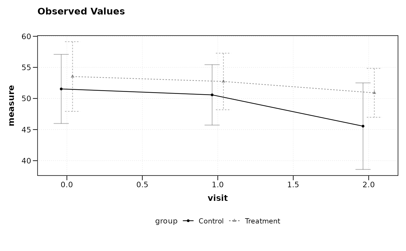
# Plot observed values by visit and group
lplot(df, measure ~ visit | group, baseline_value = 0,
cluster_var = "subject_id")
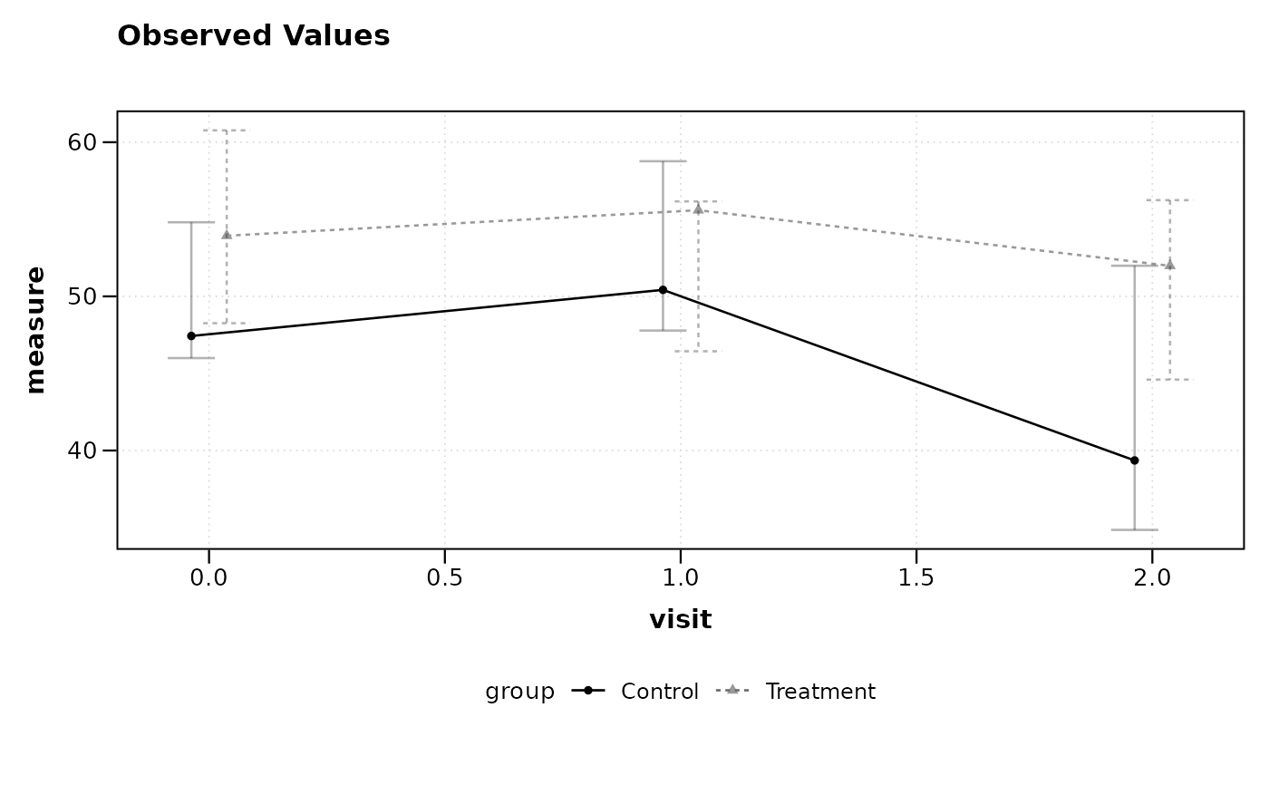
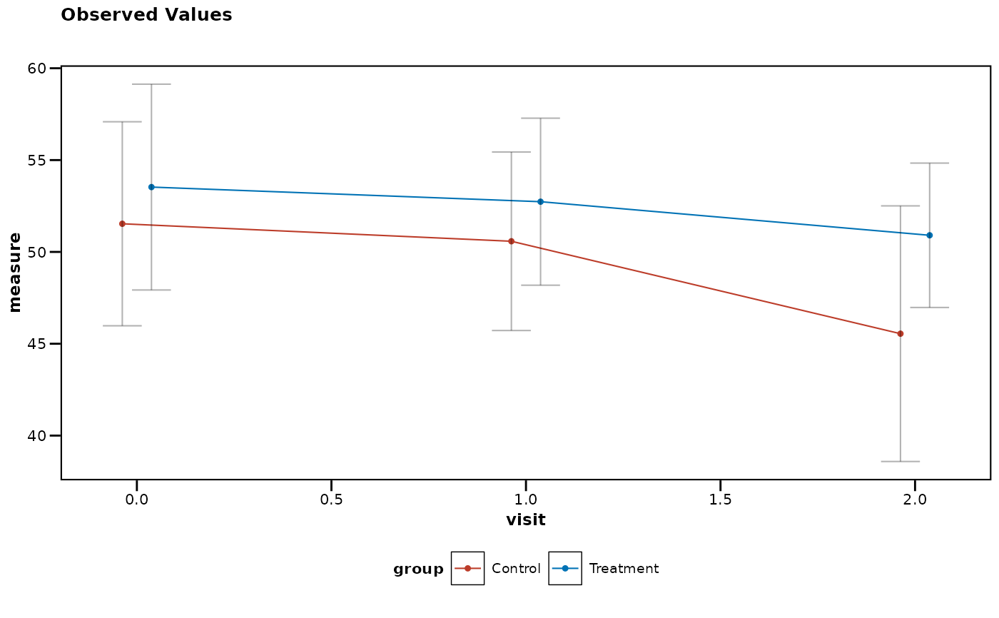
 # Plot with jittered error bars for better group separation
lplot(df, measure ~ visit | group, baseline_value = 0,
cluster_var = "subject_id", jitter_width = 0.15)
# Plot with jittered error bars for better group separation
lplot(df, measure ~ visit | group, baseline_value = 0,
cluster_var = "subject_id", jitter_width = 0.15)
 # Plot using median and IQR instead of mean and CI
lplot(df, measure ~ visit | group, baseline_value = 0,
cluster_var = "subject_id", summary_statistic = "median")
# Plot using median and IQR instead of mean and CI
lplot(df, measure ~ visit | group, baseline_value = 0,
cluster_var = "subject_id", summary_statistic = "median")
 # Plot using mean ± SE (standard error)
lplot(df, measure ~ visit | group, baseline_value = 0,
cluster_var = "subject_id", summary_statistic = "mean_se")
# Plot using mean ± SE (standard error)
lplot(df, measure ~ visit | group, baseline_value = 0,
cluster_var = "subject_id", summary_statistic = "mean_se")
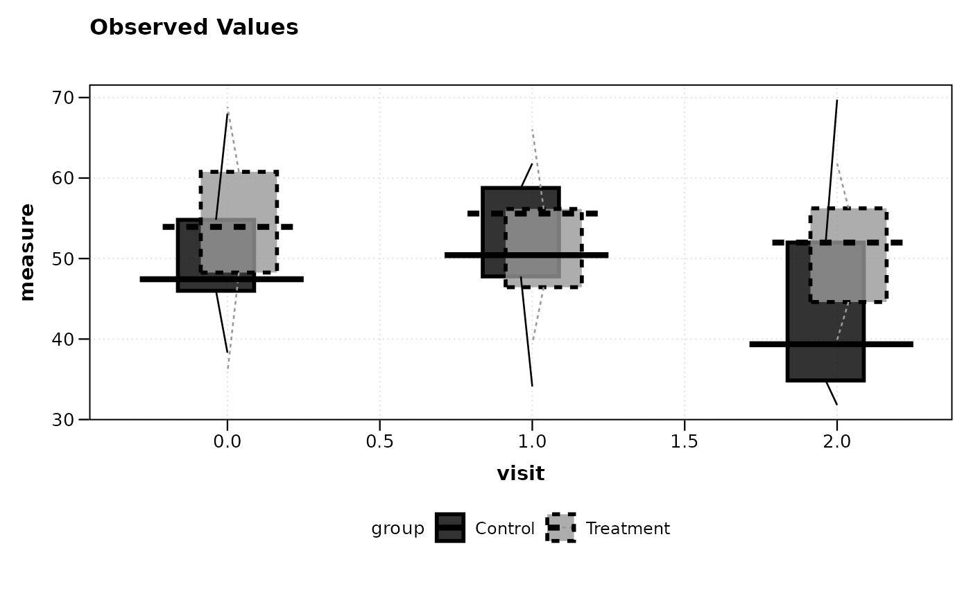
 # Plot using boxplot summary (quartiles + whiskers)
lplot(df, measure ~ visit | group, baseline_value = 0,
cluster_var = "subject_id", summary_statistic = "boxplot")
# Plot using boxplot summary (quartiles + whiskers)
lplot(df, measure ~ visit | group, baseline_value = 0,
cluster_var = "subject_id", summary_statistic = "boxplot")
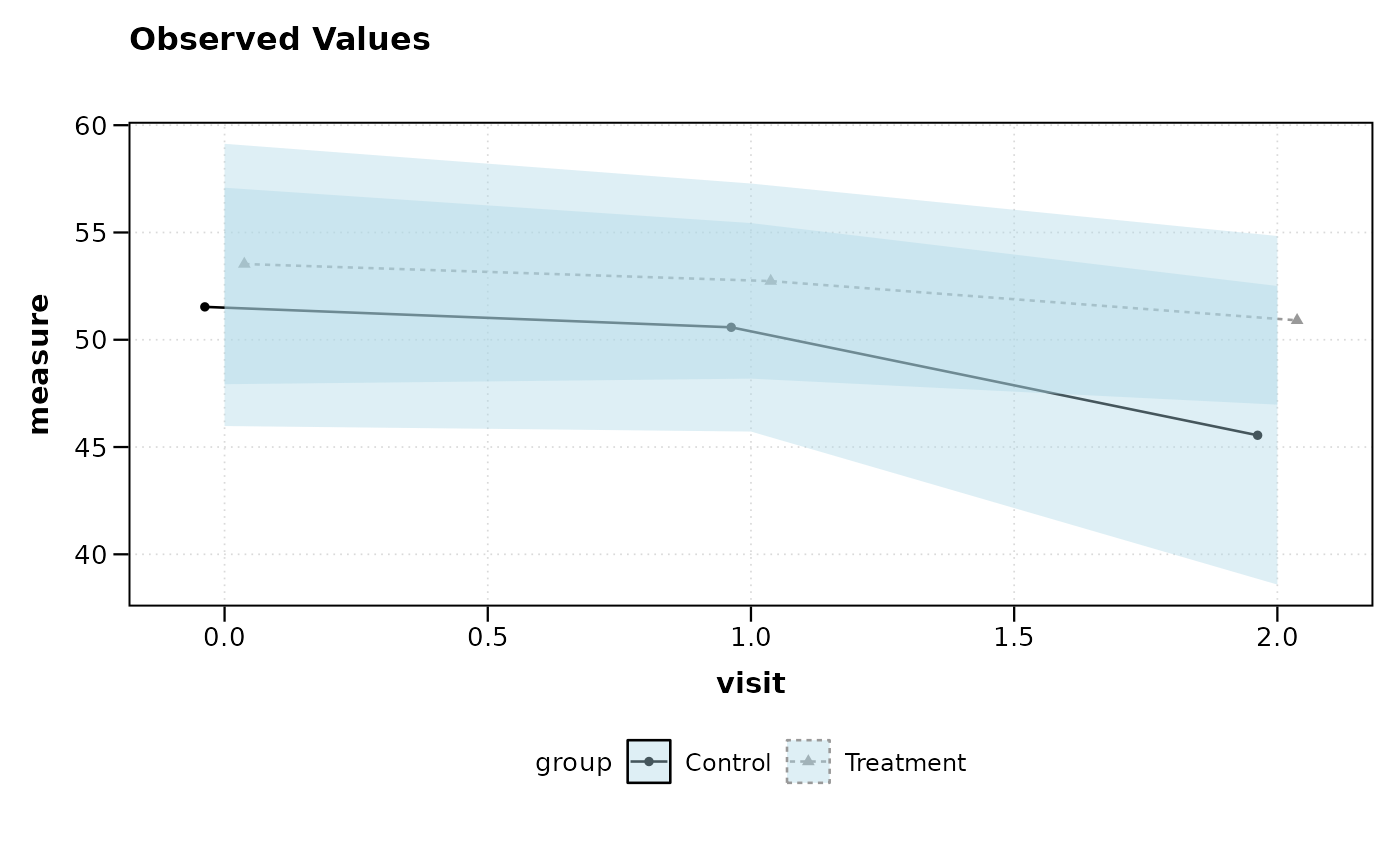
 # Customize ribbon appearance
lplot(df, measure ~ visit | group, baseline_value = 0,
cluster_var = "subject_id", error_type = "band",
ribbon_alpha = 0.4, ribbon_fill = "lightblue")
# Customize ribbon appearance
lplot(df, measure ~ visit | group, baseline_value = 0,
cluster_var = "subject_id", error_type = "band",
ribbon_alpha = 0.4, ribbon_fill = "lightblue")
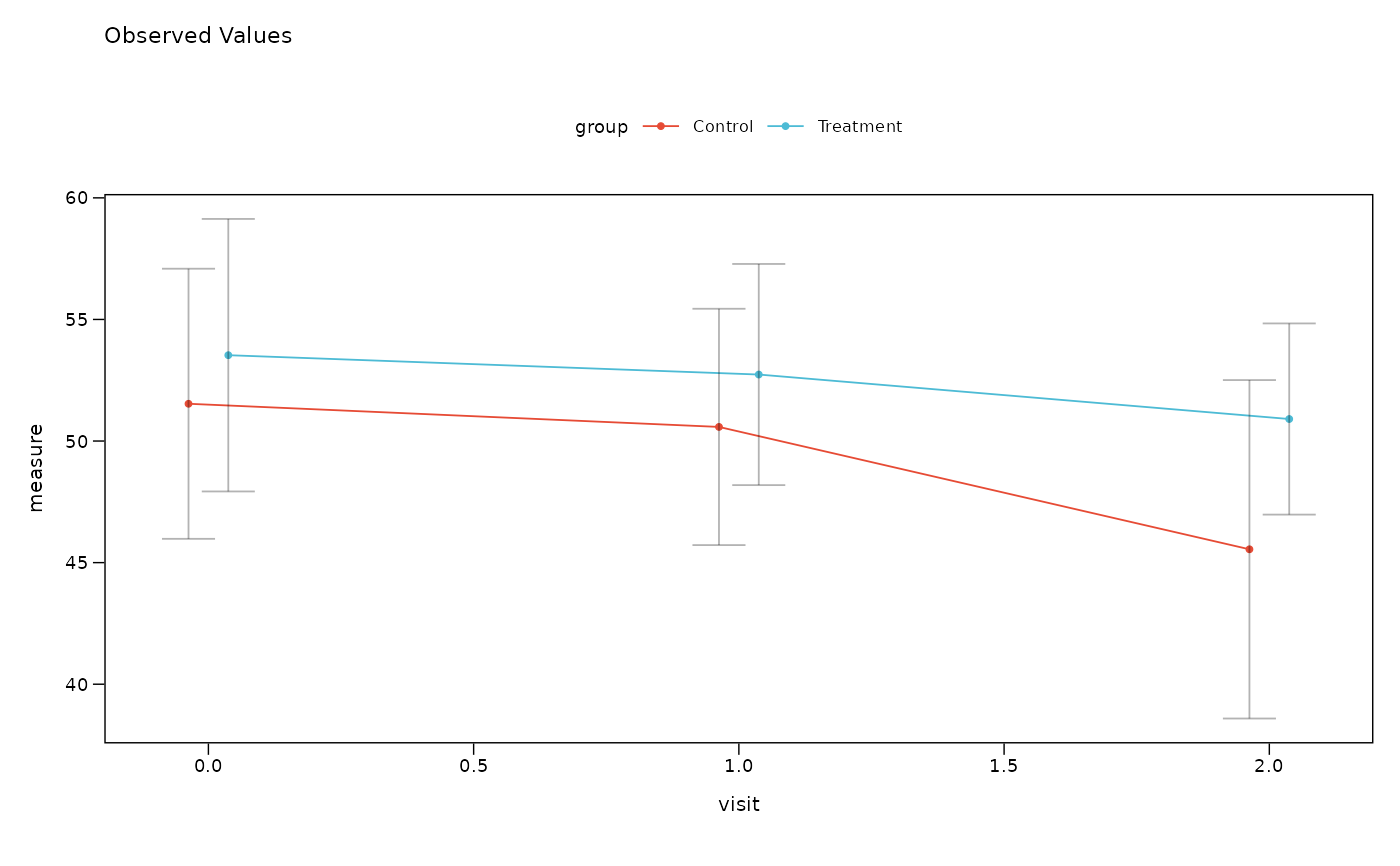
 # Apply complete journal styling (theme + colors) with single parameter
lplot(df, measure ~ visit | group, baseline_value = 0,
cluster_var = "subject_id", theme = "nejm") # NEJM theme + colors
# Apply complete journal styling (theme + colors) with single parameter
lplot(df, measure ~ visit | group, baseline_value = 0,
cluster_var = "subject_id", theme = "nejm") # NEJM theme + colors
 lplot(df, measure ~ visit | group, baseline_value = 0,
cluster_var = "subject_id", theme = "nature") # Nature theme + colors
lplot(df, measure ~ visit | group, baseline_value = 0,
cluster_var = "subject_id", theme = "nature") # Nature theme + colors
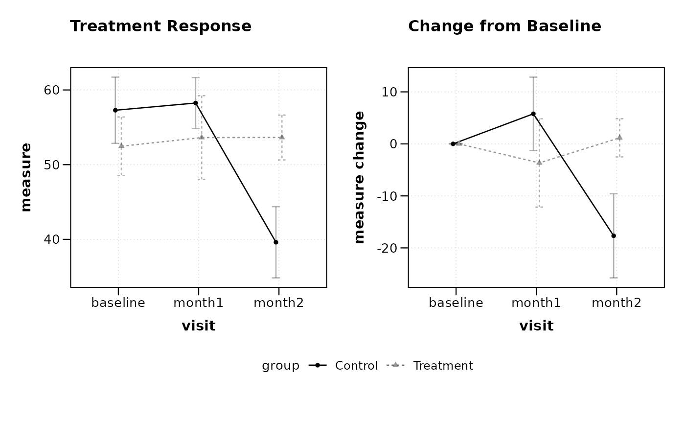
 # Example with categorical x variable
df2 <- data.frame(
subject_id = rep(1:10, each = 3),
visit = rep(c("baseline", "month1", "month2"), times = 10),
measure = rnorm(30, mean = 50, sd = 10),
group = rep(c("Treatment", "Control"), length.out = 30)
)
# Plot both observed and change values
lplot(df2, measure ~ visit | group, baseline_value = "baseline",
cluster_var = "subject_id", plot_type = "both",
title = "Treatment Response", title2 = "Change from Baseline")
# Example with categorical x variable
df2 <- data.frame(
subject_id = rep(1:10, each = 3),
visit = rep(c("baseline", "month1", "month2"), times = 10),
measure = rnorm(30, mean = 50, sd = 10),
group = rep(c("Treatment", "Control"), length.out = 30)
)
# Plot both observed and change values
lplot(df2, measure ~ visit | group, baseline_value = "baseline",
cluster_var = "subject_id", plot_type = "both",
title = "Treatment Response", title2 = "Change from Baseline")
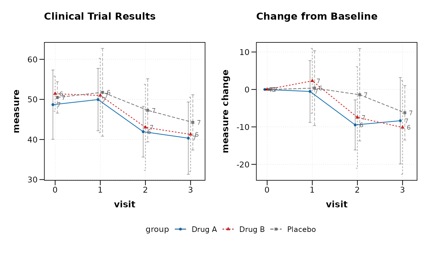
 # Clinical trial example with CDISC variables
clinical_data <- data.frame(
USUBJID = rep(paste0("001-", sprintf("%03d", 1:20)), each = 4),
AVISITN = rep(c(0, 1, 2, 3), times = 20),
AVAL = rnorm(80, mean = c(50, 48, 45, 42), sd = 8),
TRT01P = rep(c("Placebo", "Drug A", "Drug B"), length.out = 80)
)
# Clinical mode with automatic CDISC handling
lplot(clinical_data, AVAL ~ AVISITN | TRT01P,
cluster_var = "USUBJID", baseline_value = 0,
clinical_mode = TRUE, plot_type = "both",
title = "Clinical Trial Results")
# Clinical trial example with CDISC variables
clinical_data <- data.frame(
USUBJID = rep(paste0("001-", sprintf("%03d", 1:20)), each = 4),
AVISITN = rep(c(0, 1, 2, 3), times = 20),
AVAL = rnorm(80, mean = c(50, 48, 45, 42), sd = 8),
TRT01P = rep(c("Placebo", "Drug A", "Drug B"), length.out = 80)
)
# Clinical mode with automatic CDISC handling
lplot(clinical_data, AVAL ~ AVISITN | TRT01P,
cluster_var = "USUBJID", baseline_value = 0,
clinical_mode = TRUE, plot_type = "both",
title = "Clinical Trial Results")