The Formula Interface

Ronald (Ryy) G. Thomas

2026-05-11

library(zzlongplot)
library(ggplot2)

Overview

The lplot() function uses a formula interface to specify the relationship between outcome, time, and grouping variables. This design follows the convention established by base R modeling functions such as lm() and aov(), making the syntax familiar to most R users.

The general form is:

outcome ~ time | group

where each component maps to a plot element:

• outcome (left of ~): the response variable, plotted on the y-axis
• time (right of ~, before |): the independent variable, plotted on the x-axis
• group (after |): an optional grouping variable, mapped to color and linetype

The formula is parsed internally by parse_formula(), which extracts each component as a character string for downstream use in summary statistics and plot construction.

Example data

The examples below use a simulated longitudinal dataset with two treatment arms measured at five visits.

set.seed(123)
n <- 20

trial <- data.frame(
  subject_id = rep(1:n, each = 5),
  visit = rep(0:4, times = n),
  arm = rep(c("Drug", "Placebo"), each = 5 * n / 2)
)
trial$score <- 50 +
  ifelse(trial$arm == "Drug", -2.5, -0.5) * trial$visit +
  rnorm(nrow(trial), sd = 4)

Simple formula: y ~ x

The minimal formula specifies only an outcome and a time variable. This produces a single line with error bars summarising all subjects together, with no group differentiation.

lplot(trial, score ~ visit, baseline_value = 0,
      plot_type = "obs")
#> Warning: The `size` argument of `element_line()` is deprecated as of ggplot2 3.4.0.
#> ℹ Please use the `linewidth` argument instead.
#> ℹ The deprecated feature was likely used in the zzlongplot package.
#>   Please report the issue at <https://github.com/rgt47/zzlongplot/issues>.
#> This warning is displayed once per session.
#> Call `lifecycle::last_lifecycle_warnings()` to see where this warning was
#> generated.
#> Warning: The `size` argument of `element_rect()` is deprecated as of ggplot2 3.4.0.
#> ℹ Please use the `linewidth` argument instead.
#> ℹ The deprecated feature was likely used in the zzlongplot package.
#>   Please report the issue at <https://github.com/rgt47/zzlongplot/issues>.
#> This warning is displayed once per session.
#> Call `lifecycle::last_lifecycle_warnings()` to see where this warning was
#> generated.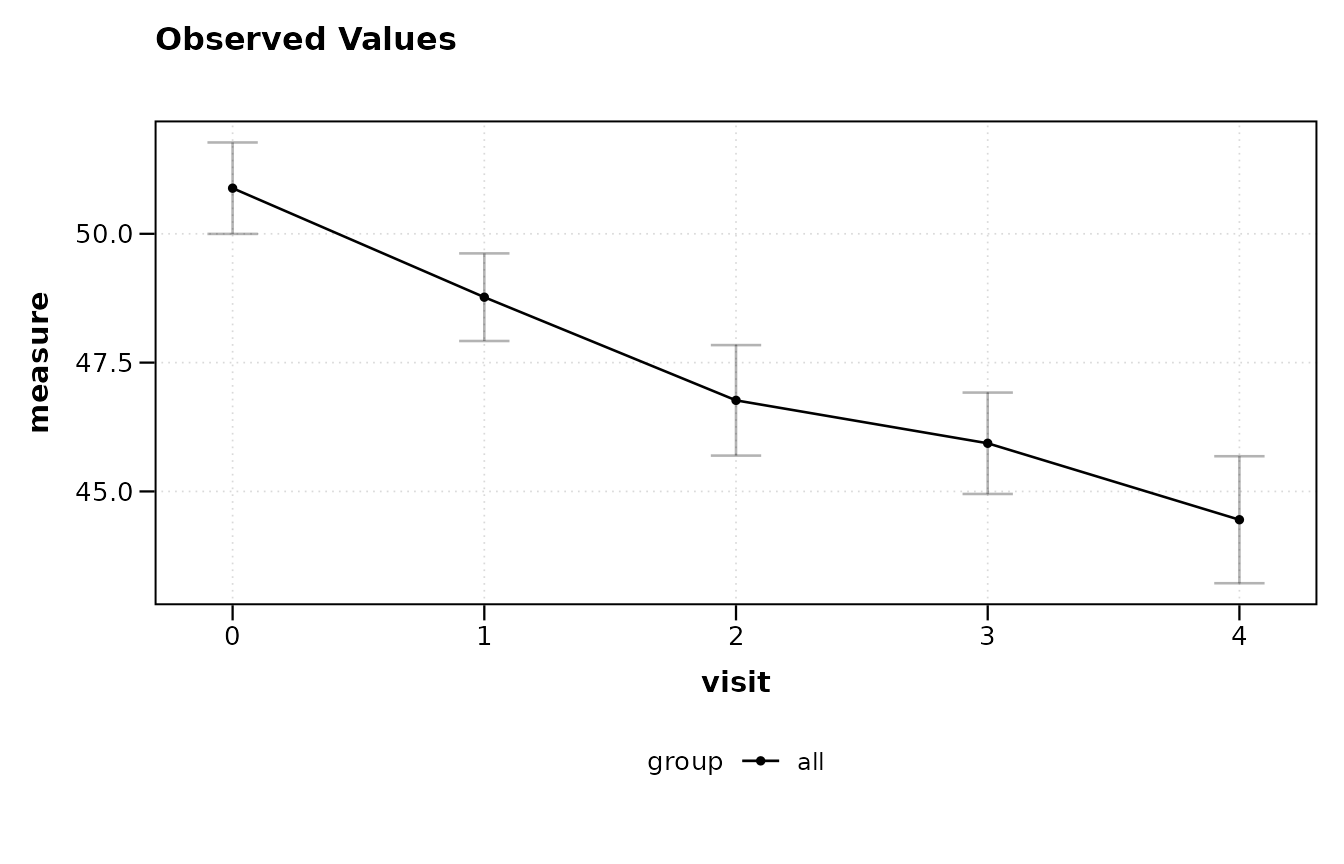

Adding a group: y ~ x | group

The pipe operator | introduces a grouping variable. Each level of the group receives its own line and color.

lplot(trial, score ~ visit | arm, baseline_value = 0,
      plot_type = "obs")

Multiple grouping variables: y ~ x | g1 + g2

When the data contain more than one factor of interest, combine them with +. The groups are concatenated into a single interaction factor for plotting.

trial$sex <- rep(c("Male", "Female"), length.out = nrow(trial))

lplot(trial, score ~ visit | arm + sex, baseline_value = 0,
      plot_type = "obs")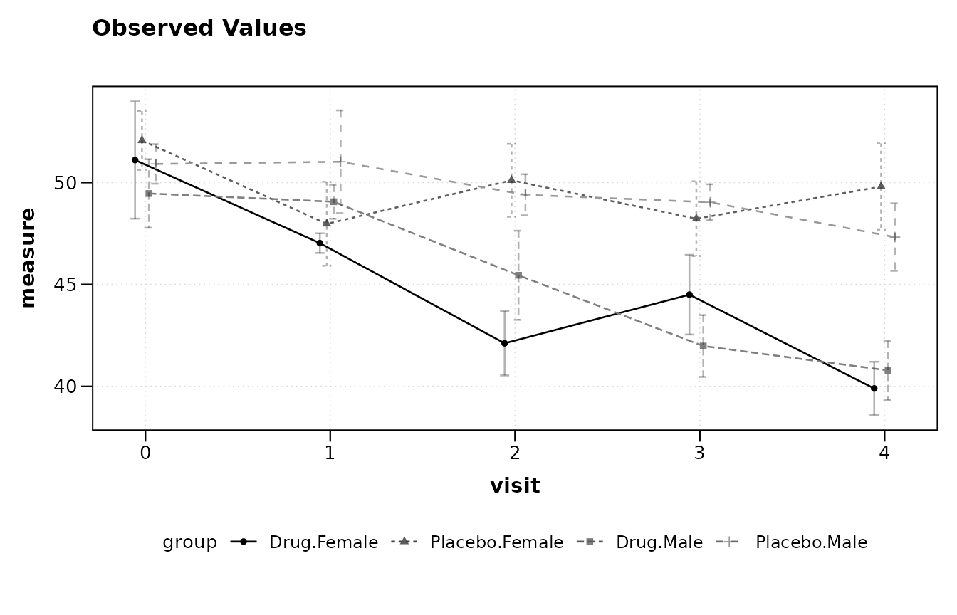

Adding facets: y ~ x | group with facet_form

Faceting is specified through a separate facet_form argument rather than through the main formula. This keeps the primary formula concise while still supporting panel layouts.

lplot(trial, score ~ visit | arm, baseline_value = 0,
      facet_form = ~ sex,
      plot_type = "obs")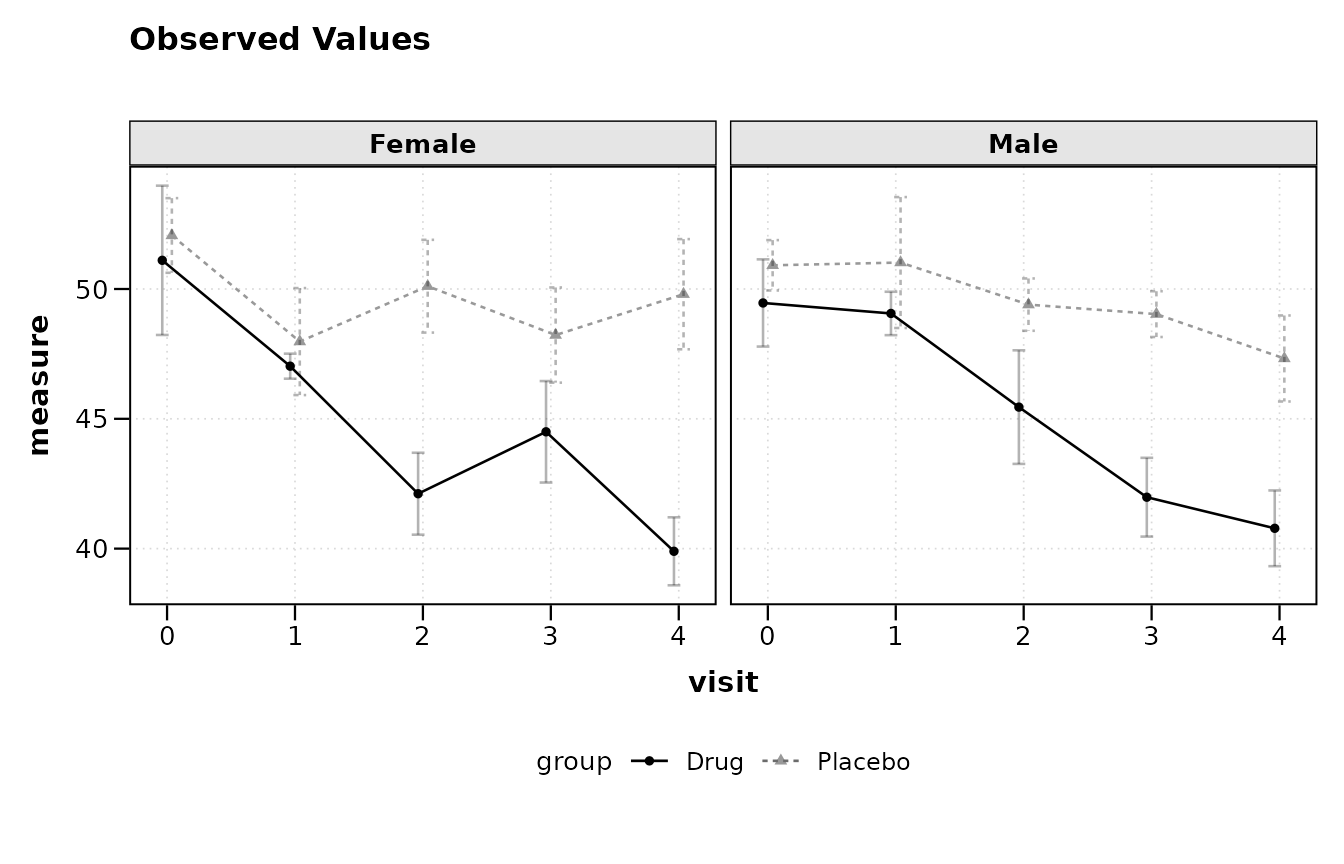

For two-dimensional faceting, use a two-sided formula:

lplot(trial, score ~ visit | arm, baseline_value = 0,
      facet_form = sex ~ site,
      plot_type = "obs")

Baseline auto-detection

When baseline_value is omitted (or set to NULL), lplot() attempts to identify the baseline visit automatically. For numeric visit variables, the minimum value is used. For character or factor visit codes, the function searches for common labels including 'bl', 'BL', 'baseline', 'screening', 'scr', 'day 0', 'week 0', 'pre', and 'visit 1'.

A message is printed to the console reporting which value was selected.

lplot(trial, score ~ visit | arm, plot_type = "obs")
#> baseline_value not specified; using 0 (minimum numeric value).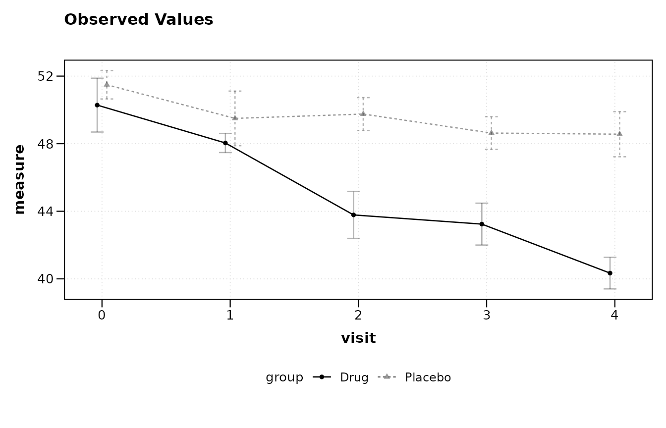

If the visit variable uses a recognised character code, the detection works the same way:

trial_char <- trial
trial_char$visit <- factor(
  trial_char$visit,
  levels = 0:4,
  labels = c("bl", "wk4", "wk8", "wk12", "wk16")
)

lplot(trial_char, score ~ visit | arm, plot_type = "obs")
#> baseline_value not specified; using 'bl'.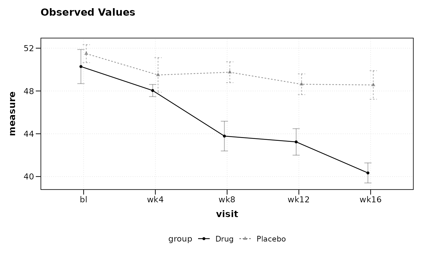

If no common baseline label is found, or if multiple candidates match (e.g., a dataset containing both 'bl' and 'baseline'), the function raises an informative error asking the user to set baseline_value explicitly.

Change from baseline

The plot_type argument controls whether observed values, change scores, or both are displayed. The formula itself does not change; the same specification drives all three plot types.

lplot(trial, score ~ visit | arm, baseline_value = 0,
      plot_type = "change")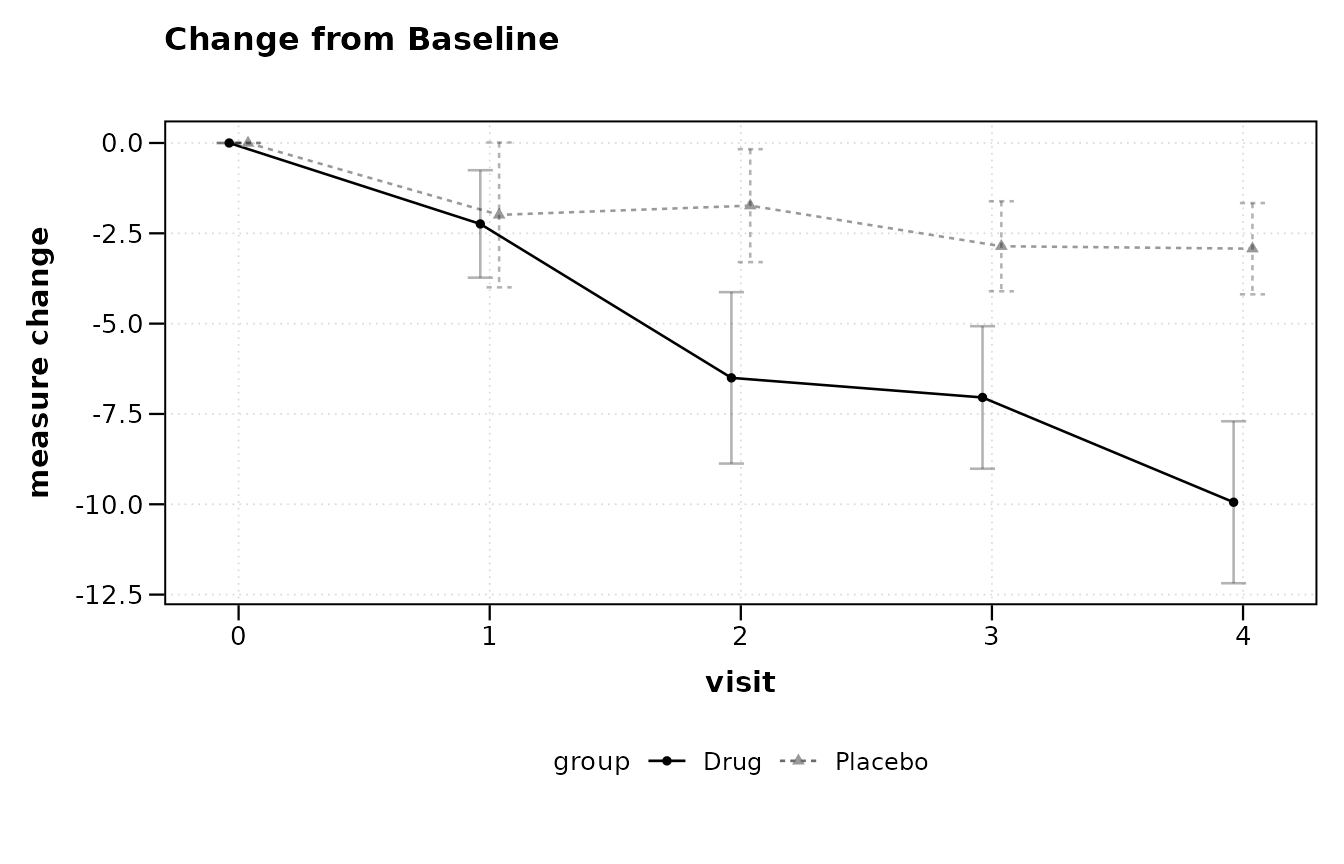

lplot(trial, score ~ visit | arm, baseline_value = 0,
      plot_type = "both")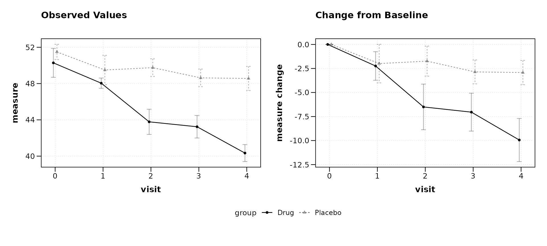

Formula parsing details

The parse_formula() function is exported and can be called directly to inspect how a formula is decomposed:

parse_formula(score ~ visit | arm)
#> $y
#> [1] "score"
#> 
#> $x
#> [1] "visit"
#> 
#> $group
#> [1] "arm"
#> 
#> $facets
#> NULL

For formulas with faceting specified in the main formula (an alternative syntax), a second ~ introduces facet variables:

parse_formula(score ~ visit | arm ~ site)
#> $y
#> [1] "score"
#> 
#> $x
#> [1] "visit"
#> 
#> $group
#> [1] "arm"
#> 
#> $facets
#> [1] "site"
parse_formula(score ~ visit | arm ~ site + region)
#> $y
#> [1] "score"
#> 
#> $x
#> [1] "visit"
#> 
#> $group
#> [1] "arm"
#> 
#> $facets
#> [1] "site"   "region"

Summary

The table below lists the supported formula patterns and their corresponding plot mappings.

Formula	y-axis	x-axis	Color/group	Facet
y ~ x	y	x	none	none
y ~ x \| g	y	x	g	none
y ~ x \| g1 + g2	y	x	g1:g2	none
y ~ x \| g ~ f	y	x	g	f
y ~ x \| g ~ f1 + f2	y	x	g	f1, f2

The facet_form argument provides an equivalent and often clearer way to specify facets separately from the main formula:

Main formula	facet_form	Result
y ~ x \| g	~ f	columns by f
y ~ x \| g	f1 ~ f2	grid: rows by f1, columns by f2