Clinical Trials with zzlongplot • zzlongplot

library(zzlongplot)
library(ggplot2)
library(dplyr)
#> 
#> Attaching package: 'dplyr'
#> The following objects are masked from 'package:stats':
#> 
#>     filter, lag
#> The following objects are masked from 'package:base':
#> 
#>     intersect, setdiff, setequal, union

Introduction

The zzlongplot package provides specialized functionality for clinical trial data visualization, with built-in support for CDISC standards, regulatory requirements, and common clinical trial analysis patterns. This vignette demonstrates how to use these clinical-specific features.

Clinical Trial Data Structure

Clinical trial data typically follows the CDISC (Clinical Data Interchange Standards Consortium) standards with specific variable naming conventions:

SUBJID: Subject identifier
AVISITN: Analysis visit number
AVAL: Analysis value (primary endpoint)
CHG: Change from baseline
TRT01P: Planned treatment
SAFFL: Safety population flag

Let’s create a realistic clinical trial dataset:

# Simulate clinical trial data
set.seed(123)
n_subjects <- 60
n_visits <- 5

clinical_data <- expand.grid(
  SUBJID = paste0("001-", sprintf("%03d", 1:n_subjects)),
  AVISITN = 0:4  # Baseline + 4 follow-up visits
) |>
  mutate(
    TRT01P = rep(c("Placebo", "Drug A 10mg", "Drug A 20mg"), length.out = n()),
    # Simulate efficacy score (higher = better)
    AVAL = case_when(
      TRT01P == "Placebo" ~ rnorm(n(), mean = 45 - AVISITN * 0.5, sd = 8),
      TRT01P == "Drug A 10mg" ~ rnorm(n(), mean = 45 - AVISITN * 1.5, sd = 7),
      TRT01P == "Drug A 20mg" ~ rnorm(n(), mean = 45 - AVISITN * 2.5, sd = 6)
    ),
    VISITN = AVISITN + 1,
    VISIT = case_when(
      AVISITN == 0 ~ "Baseline",
      AVISITN == 1 ~ "Week 4",
      AVISITN == 2 ~ "Week 8", 
      AVISITN == 3 ~ "Week 12",
      AVISITN == 4 ~ "Week 16"
    )
  ) |>
  arrange(SUBJID, AVISITN)

head(clinical_data)
#>    SUBJID AVISITN      TRT01P     AVAL VISITN    VISIT
#> 1 001-001       0     Placebo 40.51619      1 Baseline
#> 2 001-001       1     Placebo 47.53712      2   Week 4
#> 3 001-001       2     Placebo 44.94117      3   Week 8
#> 4 001-001       3     Placebo 34.99339      4  Week 12
#> 5 001-001       4     Placebo 36.69102      5  Week 16
#> 6 001-002       0 Drug A 10mg 39.73118      1 Baseline

Basic Clinical Visualization

Standard Clinical Plot

The simplest way to create a clinical trial visualization:

# Basic clinical plot with observed values
p1 <- lplot(
  clinical_data,
  form = AVAL ~ AVISITN | TRT01P,
  cluster_var = "SUBJID",
  baseline_value = 0,
  xlab = "Visit Number",
  ylab = "Efficacy Score", 
  title = "Efficacy Over Time by Treatment Group"
)
#> Warning: The `size` argument of `element_line()` is deprecated as of ggplot2 3.4.0.
#> ℹ Please use the `linewidth` argument instead.
#> ℹ The deprecated feature was likely used in the zzlongplot package.
#>   Please report the issue at <https://github.com/rgt47/zzlongplot/issues>.
#> This warning is displayed once per session.
#> Call `lifecycle::last_lifecycle_warnings()` to see where this warning was
#> generated.
#> Warning: The `size` argument of `element_rect()` is deprecated as of ggplot2 3.4.0.
#> ℹ Please use the `linewidth` argument instead.
#> ℹ The deprecated feature was likely used in the zzlongplot package.
#>   Please report the issue at <https://github.com/rgt47/zzlongplot/issues>.
#> This warning is displayed once per session.
#> Call `lifecycle::last_lifecycle_warnings()` to see where this warning was
#> generated.

print(p1)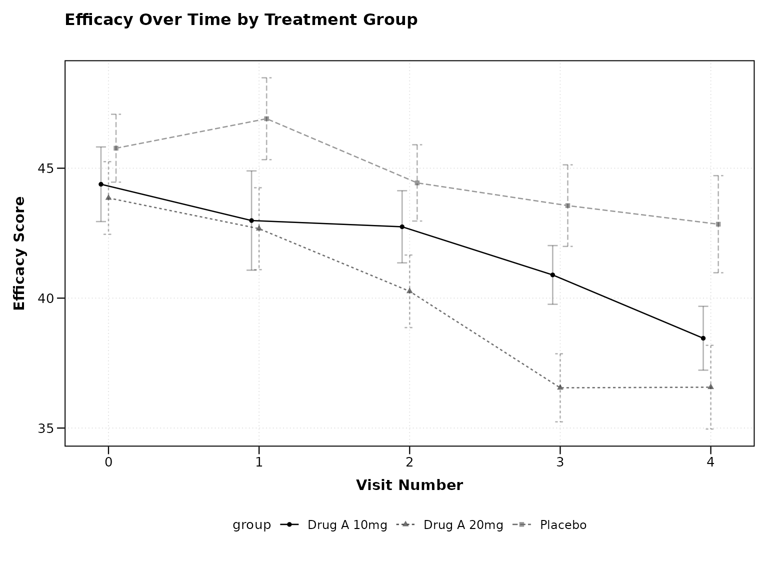

Observed and Change from Baseline

Clinical trials often require both observed values and change from baseline:

# Both observed and change plots
p2 <- lplot(
  clinical_data,
  form = AVAL ~ AVISITN | TRT01P,
  cluster_var = "SUBJID", 
  baseline_value = 0,
  plot_type = "both",
  xlab = "Visit Number",
  ylab = "Efficacy Score",
  ylab2 = "Change from Baseline",
  title = "Observed Efficacy",
  title2 = "Change from Baseline"
)

print(p2)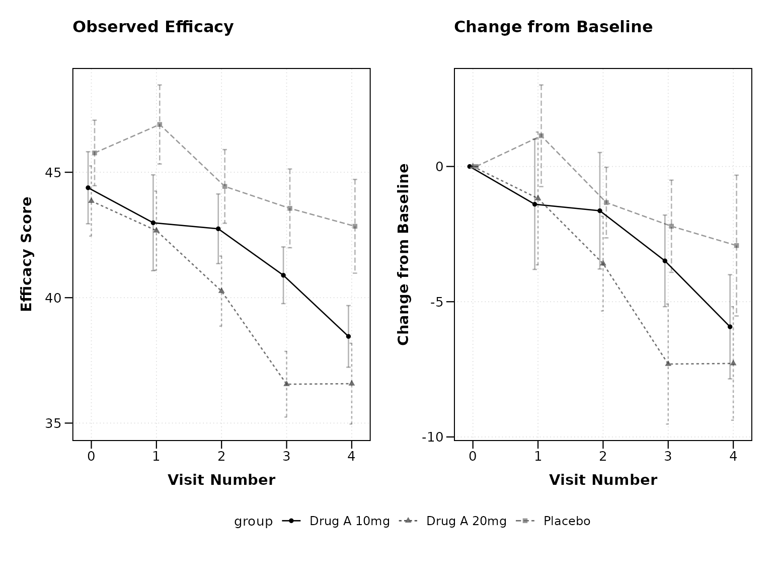

Clinical Mode Features

Enable Clinical Mode

The clinical_mode = TRUE parameter automatically applies clinical trial best practices:

# Clinical mode with all clinical defaults
p3 <- lplot(
  clinical_data,
  form = AVAL ~ AVISITN | TRT01P,
  cluster_var = "SUBJID",
  baseline_value = 0,
  clinical_mode = TRUE,
  plot_type = "both",
  title = "Clinical Trial Results",
  title2 = "Change from Baseline"
)

print(p3)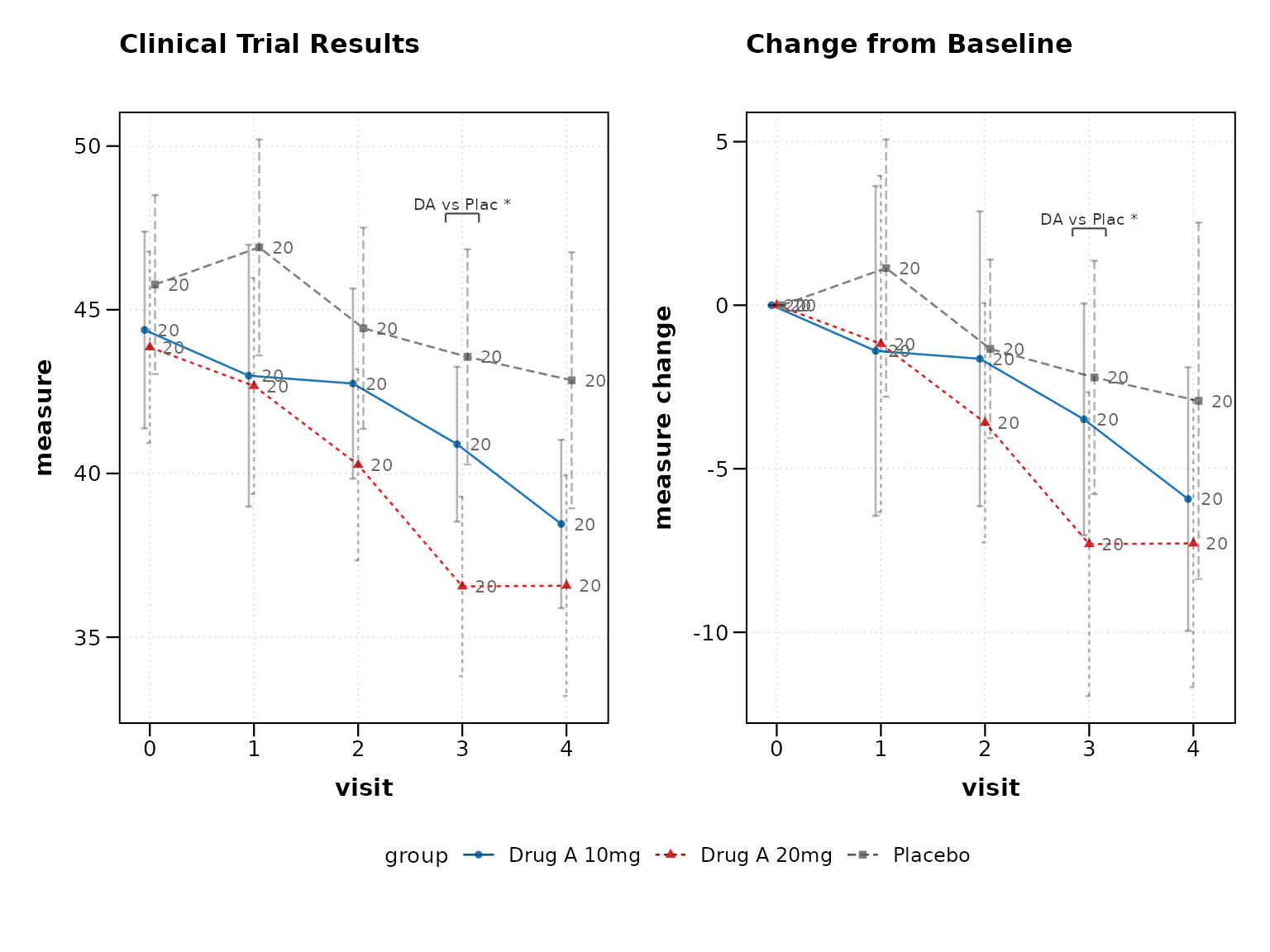

Clinical mode automatically enables: - 95% confidence intervals instead of standard error - Sample size annotations at each timepoint
- Clinical color scheme (placebo in grey, treatments in distinct colors) - Professional theme suitable for regulatory submissions

Individual Clinical Features

You can also enable clinical features individually:

# Individual clinical features
p4 <- lplot(
  clinical_data,
  form = AVAL ~ AVISITN | TRT01P,
  cluster_var = "SUBJID",
  baseline_value = 0,
  treatment_colors = "standard",     # Clinical color scheme
  confidence_interval = 0.95,        # 95% CI
  show_sample_sizes = TRUE,          # Show N at each timepoint
  error_type = "bar",               # Error bars (common in clinical)
  title = "Efficacy Analysis - Individual Features"
)

print(p4)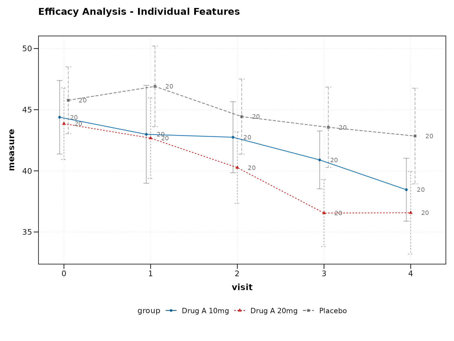

Advanced Clinical Features

Categorical Visits

Clinical trials often use visit names instead of numbers:

# Using categorical visit names
p5 <- lplot(
  clinical_data,
  form = AVAL ~ VISIT | TRT01P,
  cluster_var = "SUBJID",
  baseline_value = "Baseline",
  clinical_mode = TRUE,
  plot_type = "both",
  xlab = "Study Visit",
  title = "Efficacy by Visit",
  title2 = "Change from Baseline"
)
#> Warning in .add_pairwise_annotations(plot, stats, pw_df, x_var, y_var,
#> group_var): NAs introduced by coercion
#> Warning in max(y_vals[as.numeric(stats[[x_var]]) == xn], na.rm = TRUE): no
#> non-missing arguments to max; returning -Inf
#> Warning in .add_pairwise_annotations(plot, stats, pw_df, x_var, y_var,
#> group_var): NAs introduced by coercion
#> Warning in max(y_vals[as.numeric(stats[[x_var]]) == xn], na.rm = TRUE): no
#> non-missing arguments to max; returning -Inf
#> Warning in .add_pairwise_annotations(plot, stats, pw_df, x_var, y_var,
#> group_var): NAs introduced by coercion
#> Warning in max(y_vals[as.numeric(stats[[x_var]]) == xn], na.rm = TRUE): no
#> non-missing arguments to max; returning -Inf
#> Warning in .add_pairwise_annotations(plot, stats, pw_df, x_var, y_var,
#> group_var): NAs introduced by coercion
#> Warning in max(y_vals[as.numeric(stats[[x_var]]) == xn], na.rm = TRUE): no
#> non-missing arguments to max; returning -Inf
#> Warning in .add_pairwise_annotations(plot, stats, pw_df, x_var, y_var,
#> group_var): NAs introduced by coercion
#> Warning in max(y_vals[as.numeric(stats[[x_var]]) == xn], na.rm = TRUE): no
#> non-missing arguments to max; returning -Inf
#> Warning in .add_pairwise_annotations(plot, stats, pw_df, x_var, y_var,
#> group_var): NAs introduced by coercion
#> Warning in max(y_vals[as.numeric(stats[[x_var]]) == xn], na.rm = TRUE): no
#> non-missing arguments to max; returning -Inf
#> Warning in .add_pairwise_annotations(plot, stats, pw_df, x_var, y_var,
#> group_var): NAs introduced by coercion
#> Warning in max(y_vals[as.numeric(stats[[x_var]]) == xn], na.rm = TRUE): no
#> non-missing arguments to max; returning -Inf
#> Warning in .add_pairwise_annotations(plot, stats, pw_df, x_var, y_var,
#> group_var): NAs introduced by coercion
#> Warning in max(y_vals[as.numeric(stats[[x_var]]) == xn], na.rm = TRUE): no
#> non-missing arguments to max; returning -Inf
#> Warning in .add_pairwise_annotations(plot, stats, pw_df, x_var, y_var,
#> group_var): NAs introduced by coercion
#> Warning in max(y_vals[as.numeric(stats[[x_var]]) == xn], na.rm = TRUE): no
#> non-missing arguments to max; returning -Inf
#> Warning in .add_pairwise_annotations(plot, stats, pw_df, x_var, y_var,
#> group_var): NAs introduced by coercion
#> Warning in max(y_vals[as.numeric(stats[[x_var]]) == xn], na.rm = TRUE): no
#> non-missing arguments to max; returning -Inf

print(p5)
#> Warning: Removed 3 rows containing missing values or values outside the scale range
#> (`geom_segment()`).
#> Warning: Removed 1 row containing missing values or values outside the scale range
#> (`geom_text()`).
#> Warning: Removed 3 rows containing missing values or values outside the scale range
#> (`geom_segment()`).
#> Warning: Removed 1 row containing missing values or values outside the scale range
#> (`geom_text()`).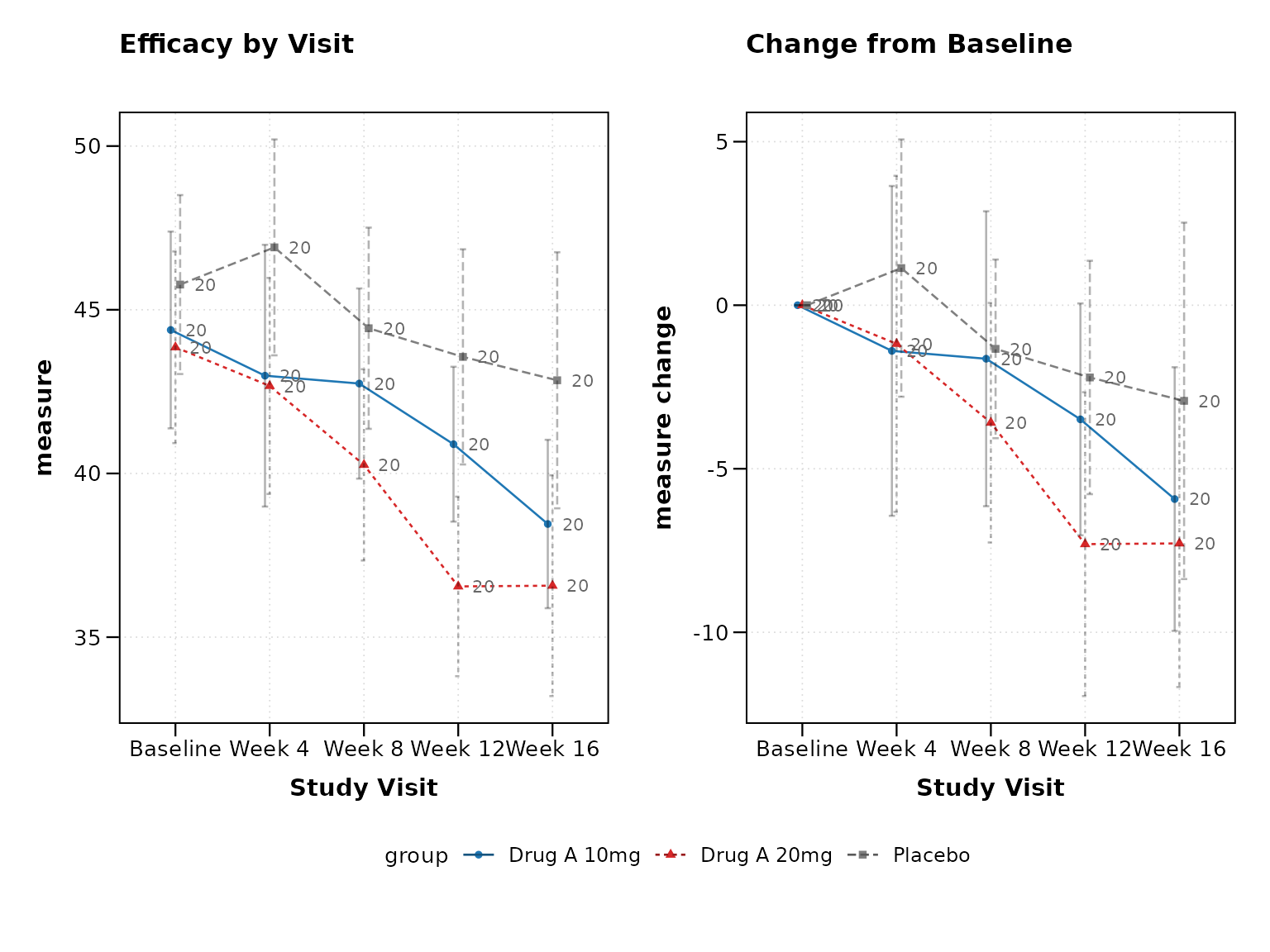

Visit Window Tolerance

Real clinical trials have visit timing variations. Handle this with visit windows:

# NOTE: visit_windows is a planned feature; the example below is
# illustrative.

# Add some visit timing variation
clinical_data_windows <- clinical_data |>
  mutate(
    VISIT_DAY = case_when(
      AVISITN == 0 ~ 0,
      AVISITN == 1 ~ round(rnorm(n(), 28, 3)),    # Target day 28 ± 3
      AVISITN == 2 ~ round(rnorm(n(), 56, 4)),    # Target day 56 ± 4  
      AVISITN == 3 ~ round(rnorm(n(), 84, 5)),    # Target day 84 ± 5
      AVISITN == 4 ~ round(rnorm(n(), 112, 6))    # Target day 112 ± 6
    )
  )

# Plot with visit windows
p6 <- lplot(
  clinical_data_windows,
  form = AVAL ~ VISIT_DAY | TRT01P,
  cluster_var = "SUBJID",
  baseline_value = 0,
  clinical_mode = TRUE,
  visit_windows = list(
    "Month 1" = c(21, 35),
    "Month 2" = c(49, 63),
    "Month 3" = c(77, 91),
    "Month 4" = c(105, 119)
  ),
  xlab = "Study Day",
  title = "Efficacy Over Time (Study Days)"
)

print(p6)

Regulatory-Ready Outputs

FDA Theme

Create plots suitable for FDA submissions:

# FDA regulatory theme
p7 <- lplot(
  clinical_data,
  form = AVAL ~ AVISITN | TRT01P,
  cluster_var = "SUBJID",
  baseline_value = 0,
  theme = "fda",
  plot_type = "both",
  title = "Figure 1.1: Primary Efficacy Endpoint",
  title2 = "Figure 1.2: Change from Baseline",
  caption = "ITT Population, LOCF imputation"
)

print(p7)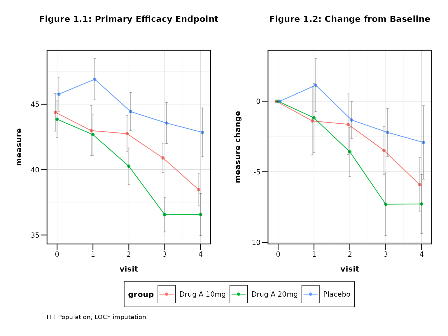

Export for Regulatory Submission

# Save in regulatory-friendly format
save_publication(p7,
  filename = "Figure_1_1_Primary_Efficacy.png",
  journal = "fda",
  width_mm = 254, height_mm = 152, dpi = 300
)

Clinical Utility Functions

CDISC Variable Detection

The package can automatically suggest appropriate formulas for your clinical data:

suggestions <- suggest_clinical_vars(clinical_data)
#> CDISC Variable Detection Results:
#> =================================
#> 
#> Suggested Formula: AVAL ~ AVISITN | TRT01P 
#> Cluster Variable: SUBJID 
#> Baseline Value: 0 
#> 
#> Detected Variables:
#>   subject_id: SUBJID
#>   visit: AVISITN, VISITN, VISIT
#>   analysis_value: AVAL
#>   treatment: TRT01P
#> 
#> Warnings:
#>   ! Using non-standard subject ID 'SUBJID'. Consider USUBJID.
#>   ! No population analysis flags detected. Consider adding SAFFL, FASFL.
print(suggestions)
#> $suggested_formula
#> [1] "AVAL ~ AVISITN | TRT01P"
#> 
#> $detected_vars
#> $detected_vars$subject_id
#> secondary 
#>  "SUBJID" 
#> 
#> $detected_vars$visit
#>  numeric1  numeric2 character 
#> "AVISITN"  "VISITN"   "VISIT" 
#> 
#> $detected_vars$analysis_value
#> primary 
#>  "AVAL" 
#> 
#> $detected_vars$treatment
#>  planned 
#> "TRT01P" 
#> 
#> $detected_vars$change
#> character(0)
#> 
#> $detected_vars$population
#> character(0)
#> 
#> 
#> $cluster_var
#> [1] "SUBJID"
#> 
#> $baseline_value
#> [1] 0
#> 
#> $warnings
#> [1] "Using non-standard subject ID 'SUBJID'. Consider USUBJID."           
#> [2] "No population analysis flags detected. Consider adding SAFFL, FASFL."

Clinical Color Palettes

Get standard clinical color palettes:

# Get clinical color palette
colors <- clinical_colors(type = "treatment", n = 3)
print(colors)
#> [1] "#7F7F7F" "#1F77B4" "#D62728"  # Grey, Blue, Red

# Use with custom styling
p8 <- lplot(
  clinical_data,
  form = AVAL ~ AVISITN | TRT01P,
  cluster_var = "SUBJID",
  baseline_value = 0,
  color_palette = colors
)

Best Practices for Clinical Trials

1. Always Show Both Observed and Change

Most clinical protocols require both perspectives:

# Best practice: Show both plots
lplot(clinical_data, AVAL ~ AVISITN | TRT01P, 
      cluster_var = "SUBJID", baseline_value = 0,
      plot_type = "both", clinical_mode = TRUE)

2. Use Confidence Intervals

95% confidence intervals are standard in clinical trials:

# Best practice: 95% confidence intervals
lplot(clinical_data, AVAL ~ AVISITN | TRT01P,
      cluster_var = "SUBJID", baseline_value = 0, 
      confidence_interval = 0.95)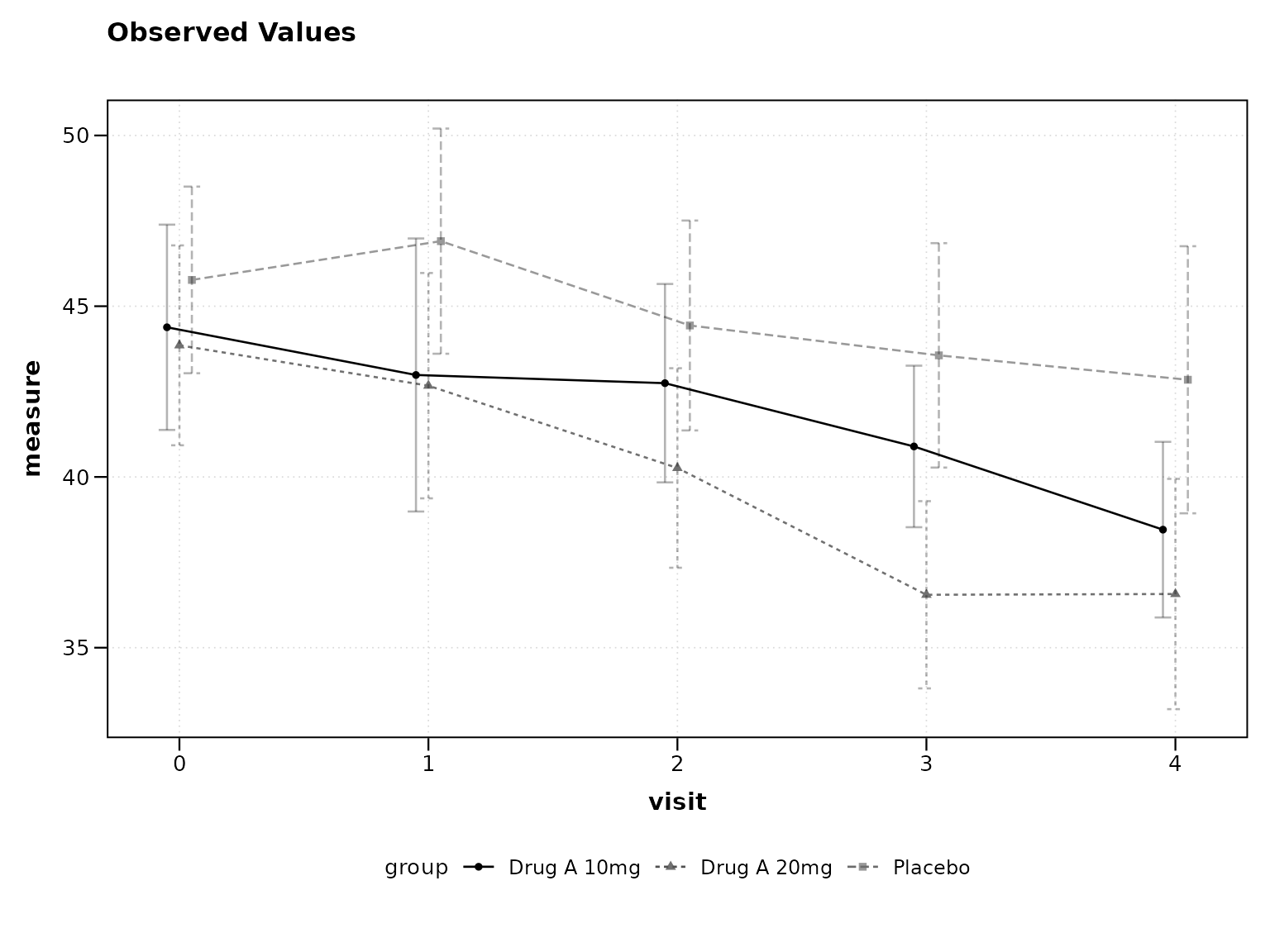

3. Include Sample Sizes

Show sample sizes to indicate data completeness:

# Best practice: Show sample sizes
lplot(clinical_data, AVAL ~ AVISITN | TRT01P,
      cluster_var = "SUBJID", baseline_value = 0,
      show_sample_sizes = TRUE, clinical_mode = TRUE)

4. Use Professional Themes

Regulatory submissions require clean, professional appearance:

# Best practice: Professional themes
lplot(clinical_data, AVAL ~ AVISITN | TRT01P,
      cluster_var = "SUBJID", baseline_value = 0,
      theme = "fda", clinical_mode = TRUE)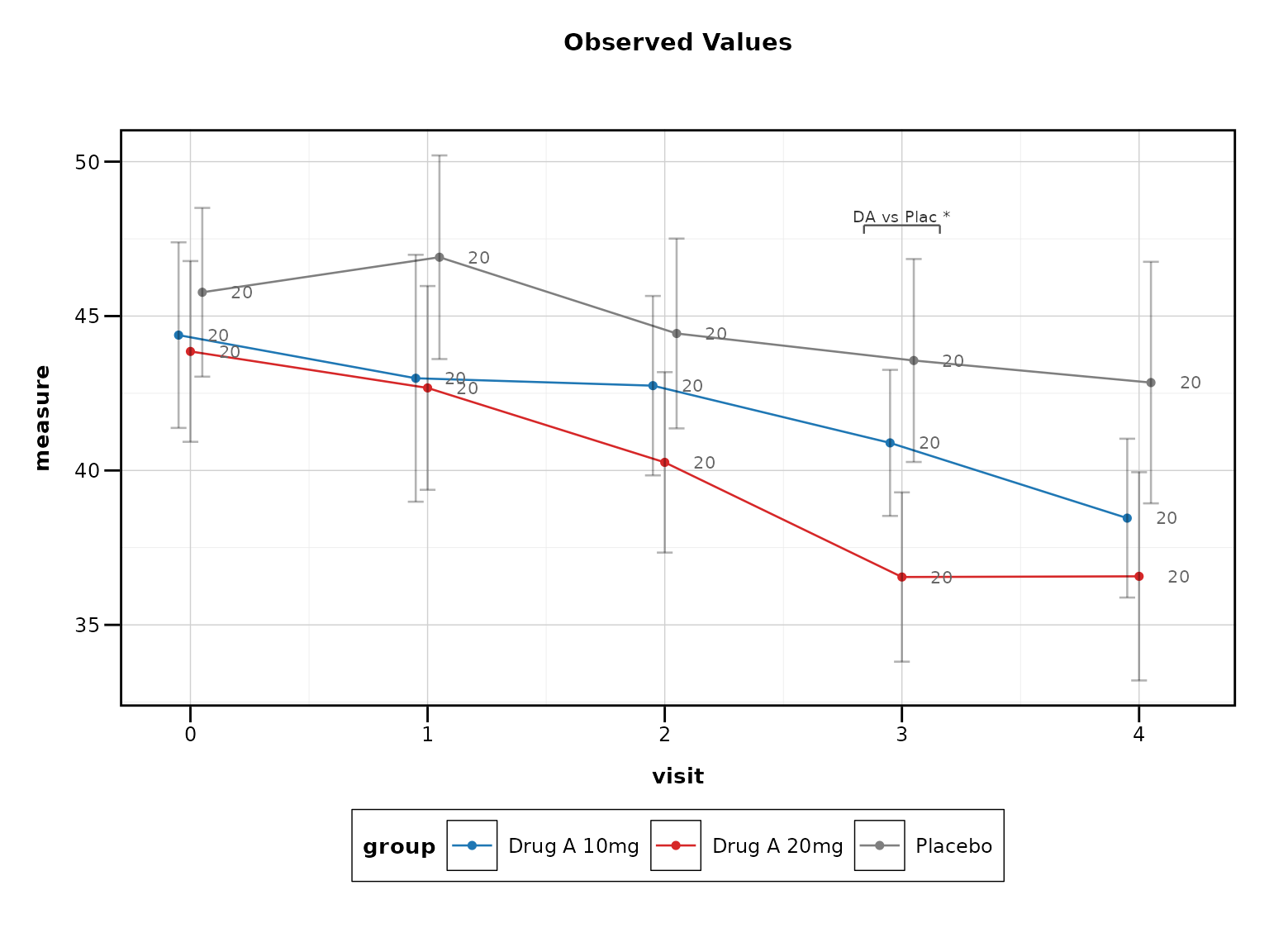

Conclusion

The zzlongplot package provides comprehensive support for clinical trial data visualization, from basic efficacy plots to regulatory-ready submissions. The clinical mode feature enables best practices with a single parameter, while individual features allow for custom requirements.

Key clinical features include: - CDISC variable recognition - Clinical color schemes and themes
- Confidence intervals and sample size annotations - Visit window handling - Regulatory output formats - Professional themes for submissions

For more examples and advanced features, see the CDISC Compliance vignette.